Introduction to the SPY-TLT Universal Investment Strategy (UIS)
This paper discusses the simple but effective method of using adaptive allocations between stock market ETFs and Treasuries to assemble a simple yet smart Investment Strategy. This method has been developed to replace the 100% switching used in normal rotation strategies like the Maximum Yield Rotation and the Global Market Rotation strategies.
The real world is just not a 100% “risk on” or “risk off” world. Most of the time, the best allocation is somewhere in between. The new method employed in this investment strategy can be adapted for nearly all types of rotation strategies and is significantly increasing the return to risk (Sharpe) ratio of such strategies.
The SPY-TLT Universal Investment Strategy is very simple but also very effective. I am sure, such a simple investment strategy will nearly always perform better than any manual asset picking.
The Universal Investment Strategy
Probably the most basic rotation investment strategy, is the switching strategy between the S&P 500 US stock market (SPY) and long duration Treasuries (TLT). The SPY-TLT ETF pair is a very interesting investment strategy, because most of the time these two ETFs profit from an inverse correlation. If there is a real stock market correction, then Treasuries like TLT have always been the assets where money flows in, rewarding holders with nice profits.
Now there are two possibilities to profit from this inverse correlation. The first is a switching strategy, which always switches to the ETF which had the best performance during the previous 3 months. This really simple switching strategy between TLT and SPY gave you a 14.8% return during the last 10 years, with twice the Sharpe ratio (return to risk) ratio of a simple SPY investment.
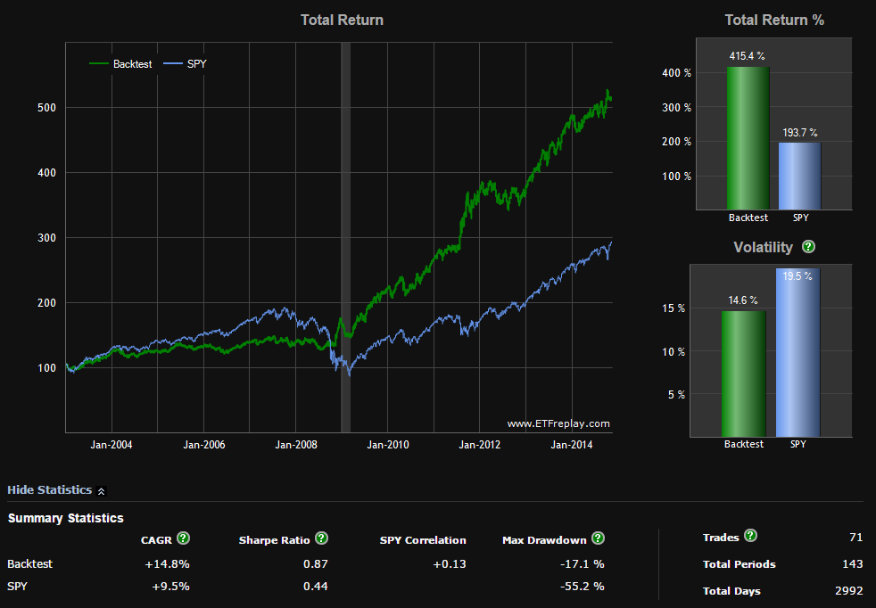
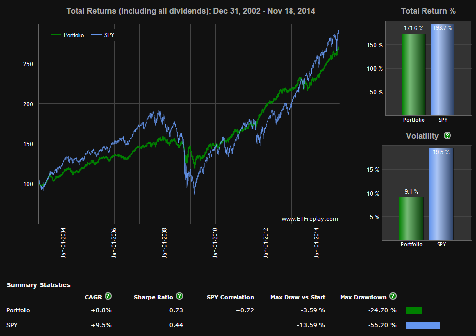
Another strategy would be to invest 50% of your money in SPY and 50% in TLT and do a monthly rebalancing. This gave you 8.8% return during the last 10 years.
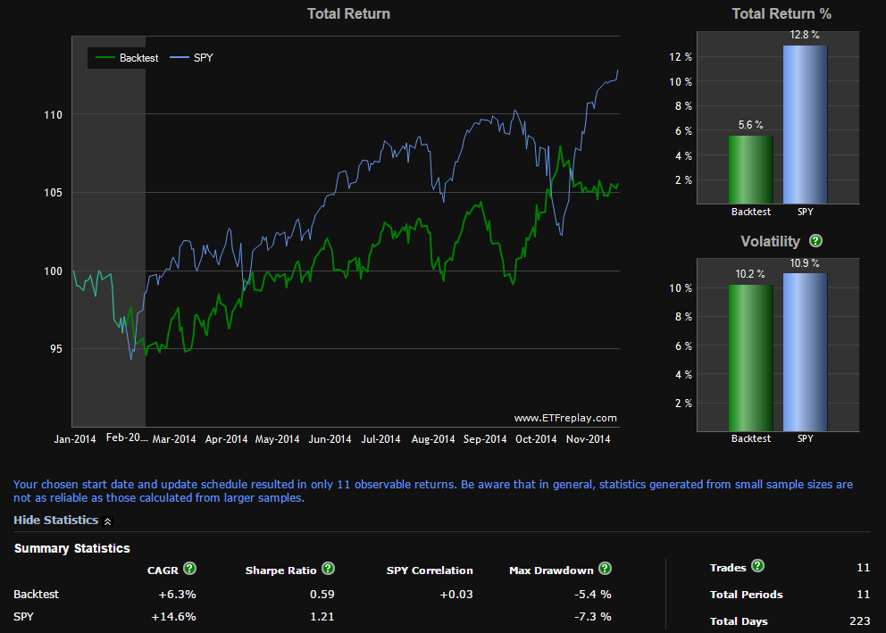
Now let’s see, how these two strategies performed the first 10 month of 2014. For quite some time we now had a sort of a sideways market. Conflicts like Syria or Ukraine made investors switch several times in “risk off” mode which favors safe haven assets like our TLT Treasury, but shortly after they switched back to “risk on” mode favoring our SPY stock market ETF. Such whipsaw market is bad for rotation strategies and as a result our SPY-TLT switching strategy only made 5.6% during the first 10 months with a Sharpe ratio of 0.59.
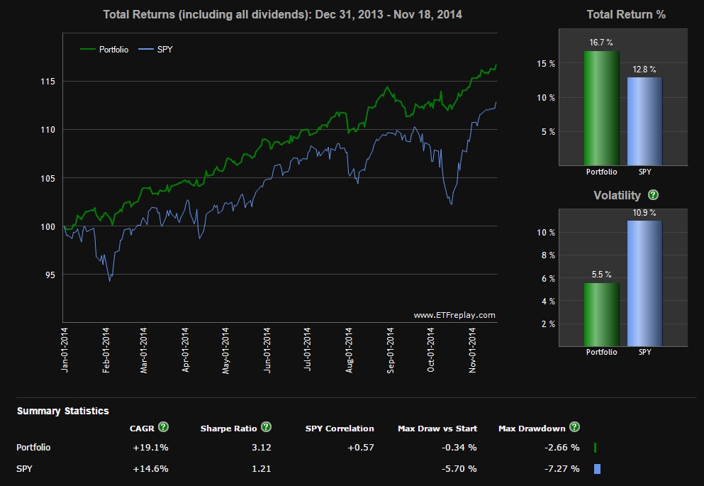
This time the much better strategy was to hold equal positions of SPY and TLT. This strategy made 16.7% during the first 10 months with an very high Sharpe ratio of 3.12.
If you analyze these two strategies, then you will quickly see which are the advantages and disadvantages of each strategy. The switching strategy did well during market periods with a strong up or down trend. In 2008 this strategy could avoid the stock market crash by switching nearly 100% to Treasuries. During sideways market periods and especially during whipsaw market periods, the switching strategy switched a lot of times too late, which resulted in an unwanted sell low and buy high strategy.
Variations of the Universal Investment Strategy
The idea for this Universal Investment Strategy was to develop a strategy which has an adaptive allocation between 0% and 100% for each ETF depending of the market situation. I am using such a strategy for quite some time with excellent results. Since 2014 the strategy invests always approximately equal parts of TLT and SPY.
The way to calculate the optimum composition is done by calculating which composition had the maximum Sharpe ratio during an optimized look back period (normally 50-80 days). During normal market periods, the maximum Sharpe ratio is not at a 100% SPY or at a 100% TLT allocation, but somewhere in between. To calculate this maximum Sharpe ratio, I loop through all possible compositions from 0%SPY-100%TLT to 100%SPY-0%TLT and calculate the resulting Sharpe ratio for the look back period.
As a result I get a curve like this (result of July 21, 2014):
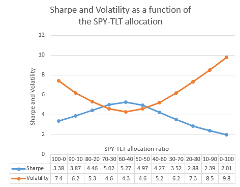
The interesting finding is, that the best combination of SPY-TLT gets with 5.27 a considerably higher Sharpe ratio then SPY (3.38) or TLT (2.01) alone. This is because the inverse correlation of the two ETFs reduces volatility or risk a lot.
On July 21, 2014 when I made this calculation, this would mean that the optimum composition for the portfolio would be 60% SPY and 40% TLT. This composition is in this case also the one with the lowest volatility.
Year to date the volatility of such a strategy is below 5%, which is less than half the volatility of SPY or 3x to 4x less compared to other markets (Europe, Emerging markets).
For my UIS strategy I tweaked the Sharpe formula a little bit. Normally the Sharpe ratio is calculated by Sharpe = rd/sd with rd=mean daily return and sd= standard deviation of daily returns. I don’t use the risk free rate, as I only use the Sharpe ratio to do a ranking. My algorithm uses the modified Sharpe formula Sharpe = rd/(sd^f) with f=volatility factor. The f factor allows me to change the importance of volatility.
If f=0, then sd^0=1 and the ranking algorithm will choose the composition with the highest performance without considering volatility.
If f=1, then I have the normal Sharpe formula.
If f>1, then I rather want to find SPY-TLT combinations with a low volatility. With high f values, the algorithm becomes a “minimum variance” or “minimum volatility” algorithm.
To get good results, the f factor should normally be higher than 1. This way you do not need to rebalance too much. In a whipsaw market, rebalancing also has the negative effect of selling low and buying high on small intermediate market corrections. This is why a system which considers only performance will not do well.
The good f factor for a system can be found by “walk forward” optimization iterations of your backtests. Normally a good value for f is about 2, but the factor changes slightly, adapting to the current market conditions.
Comparison of different SPY-TLT investment strategies (5 year)
| Strategy | 5 year CAGR | Sharpe ratio | |
| 1 | SPY-TLT UIS adaptive allocation | 18% annual return | 1.66 |
| 2 | 50% SPY- 50% TLT rebalanced monthly | 12.5% annual return | 1.31 |
| 3 | SPY – TLT monthly rotation strategy | 19% annual return | 1.19 |
It is interesting to see, that the return of such an investment strategy will be higher if market volatility is higher. So, for the low volatility period from 2000-2007 (SPY volatility of 13), the annual return was about 9%, but since then, we had an average SPY volatility of 23, which results in a much higher return for the strategy. So this means, that with such a strategy we are happy if we have a really nice 25% market correction followed by a recovery, because this means, that we can profit from the market corrections by over-weighting TLT and later on, we profit again from the recovery by over-weighting SPY.
So, in summary, a variable allocation between stock market ETFs and Treasuries has by far the best risk/return (Sharpe) ratio for this investment strategy. Fixed ratios do only perform well, when market conditions do not change. Be skeptical if somebody will sell you a strategy with a fixed allocation which is only backtested for the last few bull market years. Normally these strategies will fail when the next 2008 like bear market begins. The older methodology SPY-TLT rotation has a slightly higher return, but a much higher volatility or risk. Return alone should never be used to judge a strategy. In fact it is very simple to boost the return by using leveraged ETF replacements for SPY and TLT. But this would in no way make the strategy superior, because then also the volatility or risk will be higher by the leverage factor.
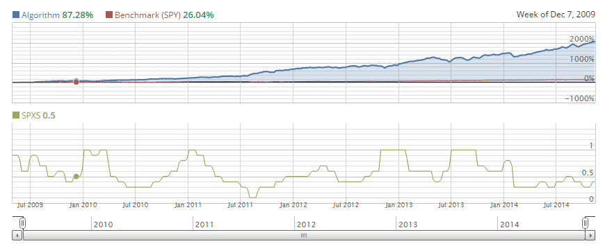
Here is a plot of the results if you use short positions of the -3x leveraged SPXS-TMV instead of SPY-TLT. The result is incredible. 2051% return for the 5.5 year period. This is a 74% annual return with a Sharpe ratio of 2.6. In the below chart, you see also a green chart which shows you the monthly SPXS allocation. The TMV allocation is always the 100%- SPXS allocation. It is interesting to see, that even if we had a bull market during this period, in average the strategy is about 50% invested in Treasuries.
Other uses for the Universal Investment Strategy
The adaptive SPY-TLT allocation strategy is also very interesting, because you can use it for different other investment strategies. In general the UIS strategy gives you the very important information, on how to position your investments between “risk on” stock market investments and “risk off” Treasuries. Instead of using this to invest directly in the SPY and TLT ETFs, you can us this allocation for a lot of other ETFs.
Here are some Investment strategies based on the calculated UIS allocation:
| Strategy | 5 year CAGR | Sharpe ratio | |
| 1 | Basic ETF strategy using SPY and TLT ETFs | 18% | 1.66 |
| 2 | Futures strategy using S&P 500 ES and UB or ZB Treasury Futures | 19% | 2.25 |
| 3 | Short positions of -3x leveraged SPXS and -3x leveraged TMV | 74% | 2.6 |
| 4 | Option strategies. Selling -2 SD SPY put options and -1SD TLT put options | About 75% on margin requirement | ?? |
Explanation of the strategies.
- This is the basic strategy which invests in the SPY and the TLT ETFs. Both are very liquid ETFs with tight spreads and low commission costs. If you have a margin account, then there is no problem to invest with a leverage of about 2x to 3x because of the low volatility of the strategy. This way you can easily have returns of up to 50% with your money.
- I like the futures strategy, because futures are the most efficient instruments to trade the S&P 500 and Treasuries. You only need about 2-4% margin to buy these futures, so in theory you could have a leverage up to 20x. Commissions are also very low. A big advantage compared to ETFs is that Futures trade nearly 24h a day. This allows you to exit your positions at a good price in case of a sudden crisis before the ETF market opens. Another advantage is, that Treasury futures don’t pay dividends. Dividend is included in the Future price and results in a capital gain when you roll the futures. For example in Switzerland this is a big advantage, because capital gains are tax free and dividends are taxed like a normal income.
In the States futures are submitted to the 60%-40% tax rule, which means that 60% of a capital gain or loss may be treated as a long-term capital gain or loss and 40% may be treated as a short-term capital gain or loss, even if the position was held for less than a year.
A disadvantage with futures is, that they usually expire after one to three months. Therefore, you have to roll (sell the old and buy the new future) them every 3 month. Another disadvantage is that one future is normally about 100’000 US$ or more. So, if you only have a small account, then futures are too big for you. - If you can short ETFs, then I would invest in the -3x leveraged equivalents of SPY and TLT. This is what I do since about 2 years. If you short these ETFs, then you are in fact long with a 3x leverage. The nice thing is, that these -3x leveraged ETFs have very big rebalancing losses and high commissions. If you short these ETFs, then you profit from these losses. This adds about 1% of free profit per month to your strategy. Both TMV and SPXS have quite low borrowing costs of normally below 3% per year. This type of strategy is also known under the name “Hedged Convexity Capture”. Most of these strategies tell you to invest in fixed ratios of -3x leveraged stock and Treasury ETFs. But attention! This worked well the last years of the bull market, but as you can backtest with the 50%SPY-50%TLT strategy, such a “fixed ratio” strategy would have resulted in a loss of near to 100% during the 2008 subprime crash.
- Another interesting strategy is selling about 1-3 standard deviations OTM (Out of the Money) put options with about a 50 day expiry on SPY and TLT. In addition to the about 82% probability of a winning month for the base SPY-TLT strategy, you invest in options with a more than 90% probability of profit. This strategy is very interesting, because even if you once sell for example the SPY put option with a loss, then you can be nearly 100% sure that the other TLT put option will return the maximum profit.
There are two advantages over normal option strategies. Normally if you calculate a probability of profit for such a “naked” short put trade, the probability is trend neutral, only depending of implied volatility. This would mean that you have a 50% probability for an ETF to go up or down. However if you add our SPY-TLT UIS basic strategy to it, then you increase the probability of profit, because you will invest with a high probability trend. The other advantage is to execute always pair trades with an inverse correlation. Together with stop loss orders, this reduces the remaining risk a lot.
This strategy has a low volatility because both options have about the same delta and therefore inverse moves. The thing which you will see, is the slow premium (i.e., theta) decay adding profit to your account. I am still testing this strategy and while I could backtest the monthly returns I was not able until now to calculate volatility or Sharpe ratios. However the volatility seems well below 5%.
Another possible option strategy is to sell ATM (At the Money) put options with an expiration of about 4-6 months. If you hold them only for about 2-3 month, then delta will not change much and such a position behaves much like a long position of SPY or TLT within about +-5% price changes of the underlying ETF. The difference to a direct investment in SPY-TLT is, that here you get the additional premium which will boost your profits. Drawback of these option strategies is the low volume of traded TLT options which sometimes results in large bid-ask spreads.
Where can I find the current signal for this new strategy (UIS)?
I have just sent it to the “all strategy subscribers” and it is also available under the “subscriber only” blog section.
For the option strategy #4, would you adjust the ratio of contracts on TLT:SPY according to the UIS ratio each month? I did well in October selling call spreads on SVXY coming out of the volatility bump, but I’d like to add a strategy for sideways markets.
Yes, I did it for 9 months like this and it proved to be very good during normal sideways markets. If a market correction happened, then I have been always more invested in TLT put options (naked short). Only when volatility is really high and there is panic in the markets, then I think you should again overweight selling OTM SPY puts even if the strategy still shows a higher TLT allocation.
Tom,
I trade the SVXY exposure via delta neutral or long biased short call/short put combinations that have worked pretty well in sideways markets. However, while they benefit from a nice wind at their back with strong theta decay, they represent stacked layers of volatility. Tread carefully, if not well managed daily one can get smacked hard.
Excuse me, I meant buying call spreads on SVXY.
We have not fully tested and can not report the edges on SVXY option combinations. I can just comment from my personal analysis that while a bull call spread may be a “cheap” way, in terms of dollars outlay, to get upside long market exposure, I would not do it in my account. I avoid paying a net theta decay tax, especially when the tax is as high as it is on SVXY. If I want to “get long” SVXY,via options, I establish a short put position, and get paid to wait.
Hi, Frank,
Given your current experience with the new adaptive allocations strategy, do you now recommend applying the adaptive allocation strategy to the original GMR and MYR strategies, or do you recommend continuing to select the single top ranked fund @ 100% for those strategies?
Yes, the new adaptive allocations are a big improvement compared to the old 100% switching. The average return to risk ratio is significantly higher.
Thank you for this. Will I be able to get the updates or will I have to pay additional ?
If you want to use TMV instead of TLT in our UIS strategy, then you do not need to do any update. It is the same strategy, you just have to calculate the new allocations. If you replace TLT by TMV, then you can use the same allocation percentages as for SPY-TLT.
If you just want to use TMV together with SPY, then have to do a small calculation to get the percentage. TMV%=TLT%/(3*spy%+TLT%)
So, 50%TLT+50%SPY = 25%TMV(short)+75%SPY
Frank,
I noticed that you didn’t suggest this substitution (TMV%=TLT%/(3*spy%+TLT%)) in the January 2015 UIS. Is it not as desirable as those you suggested?
There is no problem to replace only TLT with TMV or TMF. But with TMV I would also use SPXU. This way you have all ETFs leveraged the same way.
If I understand correctly, applying the adaptive allocation strategy to the original GMR and MYR strategies would entail applying the adaptive allocation algorithm to (a) the top-ranked ETF, and (b) EDV. What if the top-ranked ETF for the GMR and/or MYR strategies already would be EDV — would you in that case allocate 100% to EDV, or would you apply the adaptive allocation to EDV and the 2nd ranked EFT even if the 2nd would not be ranked as high as EDV?
I do not make a normal ranking anymore as before. The new algorithm has to ETF classes. The first are ETFs with positive correlation to the stock market. The second are ETFs with negative or low correlation to the stock market. Now, these are treasuries, but I could also include precious metals, dollar index, commodities or others.
Now I check all possible x%-y% combinations of ETFs in the first class together with ETFs in the second class and I will do a ranking using my modified Sharpe parameter. But even then the allocation can be 100% Treasury, because the top ranked pair would probably be 0%MDY-100%EDV.
The good thing is, that we are now flexible to add another “risk off” ETF like gold (GLD) for example. I don’t know yet, but in the future this could make sense, because both stock and treasury market have quite a high valuation, and with gold we would have an asset with low valuation in a strategy.
Frank can you please give one specific example for selling Out of the money options for month of Dec ?
For example you could sell 20 x OTM SPY put options with a strike of 195 and expiry of February 20. So, the strike is about 10% below the current SPY price. You will get 2.55$ premium.
At the same time you could sell 40 x OTM TLT put options with a strike of 115 and expiry of February 20. So, the strike is about 5% below the current TLT price and you will get 0.69$ premium.
For SPY I normally set a lower strike, because if the market crashes, then only SPY will go down. TLT normally goes down slowly. It is important to have some stop loss limits. You can set these for example at double the premium or you close the put position if the underlying ETF falls below the strike.
This is just an example. Option trading is not an exact science and there are hundreds of possibilities to do such a trade. Best is to inform you for example at http://www.tastytrade.com.
Hi Frank,
I see that in your analysis above that UIS option #3 (short 3x leverage SPXS and TMV) has the highest Sharpe ratio. Would you say that might be a better solution than using the MYR (ZIV and TMV)? I guess the simpler question is….would short SPXS provide more risk adjusted value than long ZIV?
I am trading both strategies with equal amounts of money. Both have a very similar return to risk ratios. MYRS is underperforming the last few months, but there are also quite long periods like for example August 2012-August 2013 where SPY-TLT (SPXU-TMV) was underperforming and MYRS could still profit very well from the 2-3% roll yield.
MYRS sometimes is stagnating when volatility goes up, but because volatility is mean reverting, later or sooner you will be awarded with all the summed up roll yields of the last months. I just keep MYRS for ever, as long as I see that I collect a good roll yield. You can see this at http://www.vixcentral.com
I have realized when shorting e.g. tmv, as it profits it seems that every 10% it should be closed(all shares) and then reshorted(more shares are now owned because of previous profit); otherwise the investment won’t compound.
Do you agree ?
Let me make an example. Your short position has an initial value of 100 ETFs at a price of 100 and goes slowly down to a price of 90. Now, to close you would need to buy 100 ETFs at 90 and later on to reestablish the position you would need to sell 111 ETFs at 90 to be at the initial position size again.
Why would you buy first 100 and then sell 111 at the same price. Better only sell 11 at 90. It is the same. By selling 11 at 90 you get 990$ which is your profit. Closing the whole position and then reopen it would just result in high trade costs.
So as the monthly newsletter allocation changes are we to close out profits?
e.g. spxs/tmv goes from 40/60 to 60/40 do we close out the short profits of spxs and then reshort them in addition to the new 60% spxs allocation which required more shares to be shorted ?
Never close the position. If for example you invest 100’000$ in the strategy, then you would need to sell more SPXS for 20’000$ and buy back TMV for 20’000$. If you are short 60’000 TMV and buy back TMV for 20’000$, then you are short for 40’000$
Thanks for your reply Frank, however it still makes no sense to me. If for example TMV goes down nicely over several yrs. it can never gain more than 99.99….% unless you “close: your shorted position and reshort it again with more shares.
These calculations are another example of how the return is improved if you “close” the shorted position and reshort it with all proceeds: Here are the results for shorting SPXS and shorting TMV in a 50%/50% split.
This was done on ETFReplay and they “close” out completely then reshort the position.
Monthly always: CAGR=53.5%, max DD=-19.7%, Rebalance Events=64
Monthly 3% band: CAGR=50.8%, max DD=-19.7%, RE=46 (bands are the gains obtained before “close”
Monthly 5% band: CAGR=48.8%, max DD=-17.4%, RE=32 of a position)
Monthly 10% band: CAGR=45.2%, max DD=-17.4%, RE=19
Monthly 15% band: CAGR=40.5%, max DD=-17.9%, RE=10
This data was acquired from Seeking Alpha. Scroll down to Aug.27, 9:54pm towards the bottom of the chat.
http://seekingalpha.com/article/2444425-benefits-of-short-selling-inverse-leveraged-etfs
thanks again for looking into this for me,
Rog Svensson
You are right that if you do nothing you can not gain more than 100% because the value of your TMV position goes slowly to 0. However if you keep the position always at the same level, then you can profit the same or even a little bit more as with a long TMF position of the same value.
All you have to do is to keep the position at the same value. This must be normally be made by selling some more TMV ETFs.
You don’t have to close the whole position just to open it again. This would only result in high commission costs. For a long position it is the same. You would not sell the whole position every month and then reopen it again. You just sell the difference to take profit.
Update on above analysis. I have been viewing my brkg. acct. incorrectly. I now understand why I need to just add or subtract to my initial Short to keep the acct. optimized.
Thank you Scott and Frank for your patience.
Have you done max. DD back testing for UIS spxs/tmv ? If not it would be very useful to your subscribers.
By the way I have found spxu to be better then spxs. Same returns but with more daily trading volume, tighter spreads and lower “hard to borrow” broker interest rates.
The max draw down of the -3x leveraged UIS strategy is 3x the drawdown of the unleveraged strategy. Also volatility is 3x higher. However return is more than 3x higher because you profit of the rebalancing losses. This is why you finally have a higher sharpe ratio.
Hi Frank. Very interesting strategy. I am curious about your modified sharpe ratio used for ranking. It seems that increasing the vol factor, f, will always have a favorable impact on the sharpe ratio. For example, assume we have a strategy with r = 20%, sd = 20% (both annualized). With f = 1, the sharpe is 1. If we make f = 2, then we have 20%/(20%^2) = 20%/4% = 5. This continues exponentially as we make f larger. Therefore choosing the strategy which had the best sharpe ratio using WFA will invariably choose the highest f settings. My question is whether you are defining returns and standard deviation differently such that the sharpe ratio doesnt approach infinity as f does. Any insight on this matter would be greatly appreciated.
You are right, but this modified Sharpe ratio is only used to find the best SPY-TLT allocation. It does not really matter for this, if the Sharpe is smaller or bigger.
At the end I still use the normal Sharpe ratio to check the return to risk ratio of the strategy.
I would have liked this stategy UIS back tested using spy/vustx as proxies. Vustx behaves like tlt but goes all the way back to 1990. This would help us see how it worked through the “other” great bear mkt.of the last decade and seen how your new “adaptive” hedging would have worked. The 90s l.t.treasuries had many pos. correlations periods with spy when spy was going down. for quite awhile.
Please consider further research for this strategy development especially to address.what to do when spy and its hedge are both losing money over an extended period.
Thank you in advance
I have just posted a short blog with a 20 year UIS backtest here:
https://logical-invest.com/universal-investment-strategy-20-year-backtest/
Regarding the options version of implementation, there is the added advantage of the “volatility risk premium”. Out of the money puts on S&P500 options persistently over-price downside risk and as a seller one is over-compensated which is a huge advantage. It increases the further OTM one goes and there is a lot of research to back this up. This not so clear for TLT puts and I admit that there is a dearth of research on those options.
It should be noted that the tail risk on options (absent a switching model such as UIS) is huge, often 20x or more the typical monthly premium received. I trade option full-time (I sell premium) I’m continually refining my risk-on/risk off model. Your work is fantastic, thanks.
Let’s say that I want to follow the strategy #3, and that the UIS says to allocate for instance, 20% SPY, 80% TLT. So, should I allocate then 20% TMV and 80% SPXS?
Oh, sorry, I just understood. I should short the ETF, and as it is negative, it will be long. So in my example I would need to short 20%SPXS and short 80% TMV. So my question here is: why is this different to the 3x leveraged Universal Investment Strategy? Should both strategies return the same, right?
UIS uses a sub-strategy called HEDGE that picks from TLT, GLD and short US sectors to use as a hedge. 3x only uses TMF as a hedge. So the allocations are a bit different each month. You can use QuantTrader for 1 month and really see how this works.
I bumped in this article, which I find enlightening, although a bit old.
I would like to have some guidance
1) Which tool can I use to plot Sharpe and volatility curves as function of the SPY-TLT allocation? in this graphis the Sharpe ratio calculated as rd/(sd^f) or is a traditional Sharpe?
2) let’s say that, following your instructions, I find that the optimal allocation would be 55% SPY and 45% TLT. Who does this allocation translate in the allocations of short SPXS and short TMV? Is it 55% short SPXS ans 45% short TMV?
thank you
See our QuantTrader application, which was developed after this post: https://logical-invest.com/quanttrader-application/portfolio-backtesting-builder-main-windows/
On this page you see details of the algorithm and can then test it in QuantTrader. Due to ways leveraged ETF are constructed the long SPY/TLT signals are different from short SPXS/TMV. You can create a custom strategy with any symbols you want and then backtest and optimize it.